Exploring Finance Data
This data project focuses on exploratory data analysis and various visualization techniques of stock prices. The focus is on bank stocks and to see how they progressed throughout the financial crisis all the way to early 2016.
**NOTE: This project is just meant to practice your visualization and pandas skills, it is not meant to be a robust financial analysis or be taken as financial advice. **
Getting the Data
Using pandas to directly read data from Yahoo finance using pandas!
Required Packages: pandas-datareader.
Pandas datareader allow to read stock information directly from the internet.
The Imports
from pandas_datareader import data, wb
import pandas as pd
import numpy as np
import matplotlib.pyplot as plt
import datetime
%matplotlib inline
Data
The data from the following financial institution is explored.
- Bank of America
- CitiGroup
- Goldman Sachs
- JPMorgan Chase
- Morgan Stanley
- Wells Fargo
To target the financial crisis, the data retrieved is from Jan 1st 2006 to Jan 1st 2016 for each of these banks.
A few steps to setup the data
- Use datetime to set start and end datetime objects.
- From the documentation, its se clear the ticker for each bank is ‘BAC’, ‘C’, ‘GS’, ‘JPM’, ‘MS’, ‘WFC’.
- Following the examples in documentation, it is clear that the data can be retrieved by using the following syntax.
# Example for Bank of America
BAC = data.DataReader("BAC", 'source', start=start_date, end=end_date)
Setting up dates using datetime module
start = datetime.datetime(2006, 1, 1)
end = datetime.datetime(2016, 1, 1)
Retrieving Data from all the listed bank above
# Bank of America
BAC = data.DataReader("GE", 'yahoo', start, end)

# CitiGroup
C = data.DataReader("C", 'yahoo', start, end)

# Goldman Sachs
GS = data.DataReader("GS", 'yahoo', start, end)

# JPMorgan Chase
JPM = data.DataReader("JPM", 'yahoo', start, end)

# Morgan Stanley
MS = data.DataReader("MS", 'yahoo', start, end)

# Wells Fargo
WFC = data.DataReader("WFC", 'yahoo', start, end)
Alternate for grabbing data together
# Data can also be retrieved for a list object
df = data.DataReader(['BAC', 'C', 'GS', 'JPM', 'MS', 'WFC'],'yahoo', start, end)
Creating a list of the ticker symbols (as strings) in alphabetical order for easy reference down the line.
tickers = ['BAC', 'C', 'GS', 'JPM', 'MS', 'WFC']
Combing all the individual dataframes into a single dataframe.
The concat method from pandas, pd.concat is used to concatenate the bank dataframes together into a single data frame called bank_stocks here. Set the keys argument equal to the tickers list. The dataframes are concatenated as columns by setting argument axis=1.
bank_stocks = pd.concat([BAC, C, GS, JPM, MS, WFC],axis=1,keys=tickers)
Setting the column name levels. This will make it easier to differentiate the data of different banks.
bank_stocks.columns.names = ['Bank Ticker','Stock Info']
Check the head of the bank_stocks dataframe to see how the data looks and if concatenation is done as desired.
bank_stocks.head()
Before continuing to explore that data, it is necessary to get familiar with the following pandas functionality
-
Multilevel Indexing: Refer to the documentation on Multi-Level Indexing here
-
Slicing (Getting cross sections of the dataframe): Using .xs.
Exploratory Data Analysis
Asking some basic question.
What is the max Close price for each bank’s stock throughout the time period?
bank_stocks.xs(key='Close',axis=1,level='Stock Info').max()
Bank Ticker
BAC    324.000000
C      564.099976
GS     247.919998
JPM     70.080002
MS      89.300003
WFC     58.520000
dtype: float64
What are the returns of each bank’s stock?
Creating a new dataframe to contain the returns for each bank’s stock.
Returns are typically defined by:
\(r*t = \frac{p_t - p*{t-1}}{p*{t-1}} = \frac{p_t}{p*{t-1}} - 1 \)
returns = pd.DataFrame()
The pandas method pct_change()can be used on the Close column to create a column representing this return value. Creating a for loop that loopes through each Bank Stock Ticker such that it creates the returns column for each back makes things faster.
for tick in tickers:
    returns[tick+' Returns'] = bank_stocks[tick]['Close'].pct_change()
returns.head()
| BAC Returns | C Returns | GS Returns | JPM Returns | MS Returns | WFC Returns | |
|---|---|---|---|---|---|---|
| Date | ||||||
| 2006-01-03 | NaN | NaN | NaN | NaN | NaN | NaN |
| 2006-01-04 | -0.001414 | -0.018462 | -0.013812 | -0.014183 | 0.000686 | -0.011599 |
| 2006-01-05 | -0.002548 | 0.004961 | -0.000393 | 0.003029 | 0.002742 | -0.001110 |
| 2006-01-06 | 0.006812 | 0.000000 | 0.014169 | 0.007046 | 0.001025 | 0.005874 |
| 2006-01-09 | -0.002537 | -0.004731 | 0.012030 | 0.016242 | 0.010586 | -0.000158 |
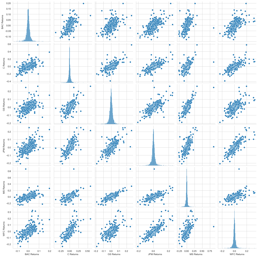
Getting the overview of which stock stands out why should infer further steps
This can be done by creating a pairplot using seaborn of the returns dataframe.
#returns[1:]
import seaborn as sns
sns.pairplot(returns[1:])
When does each bank stock has the best and worst single day returns?.
# Worst Drop
returns.idxmin()
BAC Returns   2008-04-11
C Returns     2009-02-27
GS Returns    2009-01-20
JPM Returns   2009-01-20
MS Returns    2008-10-09
WFC Returns   2009-01-20
dtype: datetime64[ns]
Note: 3 of the banks share the same day for the worst drop.
On further investigation (by which I mean google search)
2009-1-20 is (January 20th) the Inauguration day in the US.`
# Best Single Day Gain
returns.idxmax()
BAC Returns   2009-03-10
C Returns     2008-11-24
GS Returns    2008-11-24
JPM Returns   2009-01-21
MS Returns    2008-10-13
WFC Returns   2008-07-16
dtype: datetime64[ns]
Note: Citigroup and Goldman Sachs Group share the date for best single day returns.
Reason: Unclear.
Background on Citigroup’s Stock Crash available here
Which stock looks the riskiest over the entire time period?
A quick look at the standard deviation of the returns should reveal this.
returns.std()
BAC Returns    0.019775
C Returns      0.038672
GS Returns     0.025390
JPM Returns    0.027667
MS Returns     0.037819
WFC Returns    0.030238
dtype: float64
Citigroup looks the riskiest and Morgan Stanley is a close second.
Which looks the riskiest for the year 2015?
returns.loc['2015-01-01':'2015-12-31'].std()
BAC Returns    0.014076
C Returns      0.015289
GS Returns     0.014046
JPM Returns    0.014017
MS Returns     0.016249
WFC Returns    0.012591
dtype: float64
Very similar risk profiles, but Morgan Stanley is the riskiest while Citigroup is the second riskiest.
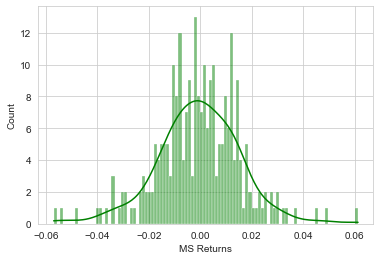
Exploring return in 2015 for Morgan Stanley
sns.histplot(returns.loc['2015-01-01':'2015-12-31']['MS Returns'],color='green',bins=100,kde=True)
Looking into return in 2008 for CitiGroup
sns.histplot(returns.loc['2008-01-01':'2008-12-31']['C Returns'],color='red',bins=100)

More Visualization
A lot of this project focuses on visualizations. Feel free to use any of your preferred visualization libraries to try to recreate the plots as described, seaborn, matplotlib, plotly and cufflinks, or just pandas.
Additional Import for Visualization
  import matplotlib.pyplot as plt
  import seaborn as sns
  sns.set_style('whitegrid')
  %matplotlib inline

  # Optional Plotly Method Imports
  import plotly
  import cufflinks as cf
  cf.go_offline()
Creating a line plot showing Close price for each bank for the entire index of time.
Using a for loop will get all the banks.
  for tick in tickers:
      bank_stocks[tick]['Close'].plot(figsize=(12,4),label=tick)
  plt.legend()

Clearly late 2008 is when the stocks take a significant fall.
Alternate to using for loops, using cross-sections - .xs should also the trick.
bank_stocks.xs(key='Close',axis=1,level='Stock Info').plot()
Imports for plotly
Plotly does interactive plots.
from plotly import __version__
from plotly.offline import download_plotlyjs, init_notebook_mode, plot, iplot

import cufflinks as cf

init_notebook_mode(connected=True)
cf.go_offline()
Interactive timeseries plot
bank_stocks.xs(key='Close',axis=1,level='Stock Info').iplot()
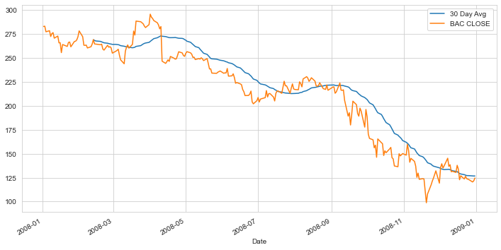
Moving Averages
Analyzing the moving averages for these stocks in the year 2008.
Plot the rolling 30 day average against the Close Price for Bank Of America’s stock for the year 2008
  plt.figure(figsize=(12,6))
  BAC['Close'].loc['2008-01-01':'2009-01-01'].rolling(window=30).mean().plot(label='30 Day Avg')
  BAC['Close'].loc['2008-01-01':'2009-01-01'].plot(label='BAC CLOSE')
  plt.legend()
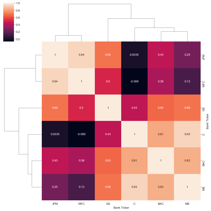
Creating a heatmap of the correlation between the stocks’ Close Price.
sns.heatmap(bank_stocks.xs(key='Close',axis=1,level='Stock Info').corr(),annot=True)

Creating a clustermap to cluster the correlations together
sns.clustermap(bank_stocks.xs(key='Close',axis=1,level='Stock Info').corr(),annot=True)
Reference jupyter notebook.