Overview

This thesis deals with the post-processing of the results obtained from a topology optimization algorithms which outputs the result as a 2D image. A suitable methodology is discussed where this output 2d geometry is processed and converted into an CAD geometry all while minimizing deviation in geometry, compliance and volume fraction while validating the results. All the programming is done in MATLAB and it uses an image based post-processing approach. The proposed workflow is tested on several numerical examples to assess the performance, limitations and numerical instabilities.

Contents

1. Background
1. Introduction
2. Problem Definition
2. Methodology
1. Topology Optimization
2. Geometry Smoothing
3. Geometry Extraction
3. Results
1. Material Properties
2. MBB Beam
3. T Beam
4. Additional Details
1. Result Metrics
2. Limitations
3. Outlook

Background

Introduction

Topology Optimization (TO) is a mathematical methodology that optimizes a material domain within a prescribed design space, subject to predefined requirements and boundary conditions such that the resulting domain meets a prescribed set of goals. TO can help greatly reduce the lead time of the component all while developing a component suited for a particular objective and also help in reducing the amount of material used in the manufacture of the component.

Problem Definition

To begin with, a simple TO code will be much easier to manipulate compared to huge commercial softwares. One such code is the popular 88-line MATLAB code which is an ideal starting point as it supports multiple load-cases, is mesh independent and is most importantly a fast solver. This code is also short and is validated by the numerous publications which support it as one of the best codes to understand how TO works. However, this code has its limitations; it can only solve 2D optimization problems and uses only bilinear quad-elements in its FE formulation. The optimized result from the code is in the form of a black-and-white image which needs to be manipulated to make it more suitable to our purposes.

This thesis deals with the formulation of a methodology or a workflow to post-process the resulting geometry from the 88-line code to make it ready for production in as little time as possible. TO geometries are usually subjected to post-processing as there might be the presence of rough surfaces, jagged edges or intermediate densities. If these rough edges end up in the final geometry they can cause stress concentrations or even decrease the fatigue life of the structure. Hence, a faster and an efficient way to post-process results is needed to make way in a much smoother and rapid product/prototype development.

Methodology

The outcome of the literature study definitively showed that the most prominent way of resolving these problems consists of three phases which are combined under a singular approach called 'Structural Design Optimization' The three phases are listed and explained in detail below.

1. Topology Optimization
2. Geometry Smoothing
3. Geometry Extraction

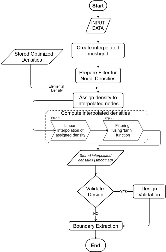
The workflow formulated is adapted from "Structural Design Optimization" concept. A flowchart depicting the generalized workflow can be seen in the figure below.

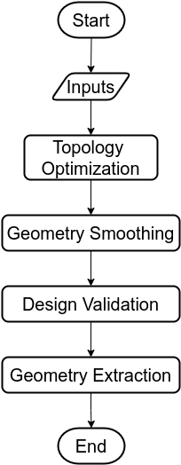
The entire workflow can be divided into three major phases excluding TO. The process begins with the input definitions being used for TO whose results along with the same inputs are shared with the next phase i.e. geometry smoothing. The smoothed geometry is then validated and finally geometry is extracted.

Topology Optimization

The TO problem in this thesis is a compliance minimization problem under a volume constraint. The generalized TO problem to solve the compliance minimization problem can be seen in the equation below.

where C is compliance, V(x) is current volume fraction, V0 is maximum volume fraction and V̄ is the target volume fraction.

The volume fraction V(x) is calculated by taking the arithmetic mean of the elemental densities, see the equation below.

\begin{equation} V(\boldsymbol{x}) = \frac{\sum_{e=1}^{n_e} \bar{x}_{e}}{n_e} \end{equation}

The 88-line code TO solver is setup to solve the above compliance minimization problem. This solver code is modified with the following few additions.

• Compliance Computation
• Compute & visualize von Mises Stresses
• Heaviside Filter

Compliance Computation

The compliance calculations were done using the following equations. For a single load case the total compliance is calculated using

\begin{equation} C({x}) = {u}^{T}{K}{u} \end{equation}

And when the geometry is subjected to more than one static load, the net compliance is the sum of n compliances due to each individual load and is computed using

\begin{equation} C({x}) = \sum_{i=1}^{n} {U}_{i}^{T}{K}_{i}{U}_{i} \end{equation}

Heaviside Filter

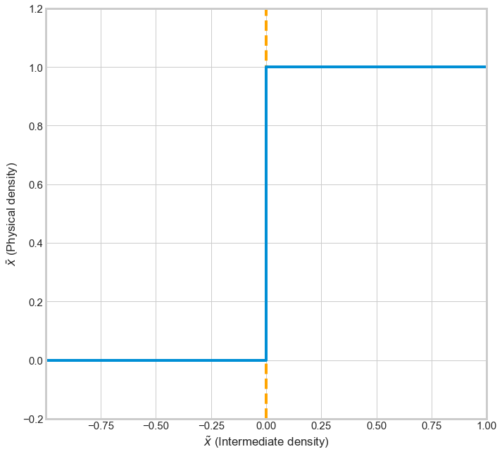
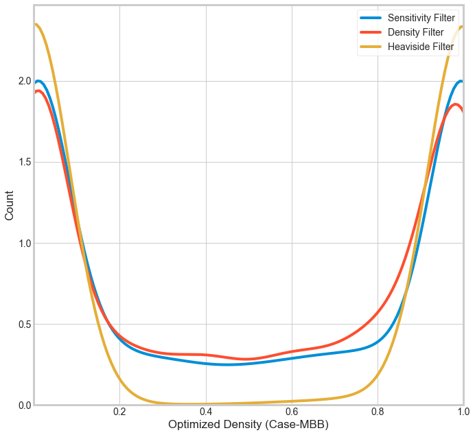
The Heaviside filter is a density filter with Heaviside step function to help move intermediate densities i.e., grey values to either one or zero when the values lie between zero and one. There are two benefits for using this filter, one is to obtain a minimum length scale in the optimized design which helps avoid the formation of any features less than the minimum value and the second is to obtain black-and-white solutions. The behavior of heaviside function and its effect on density distribution are shown in the figures below.

Note: For a detailed description and mathematical implementation on the computation of von Mises stresses, refer to Appendix A in the thesis report.

Geometry Smoothing

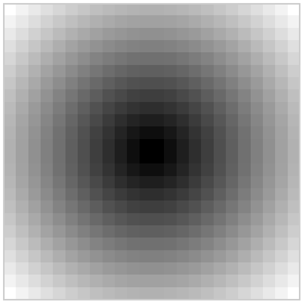
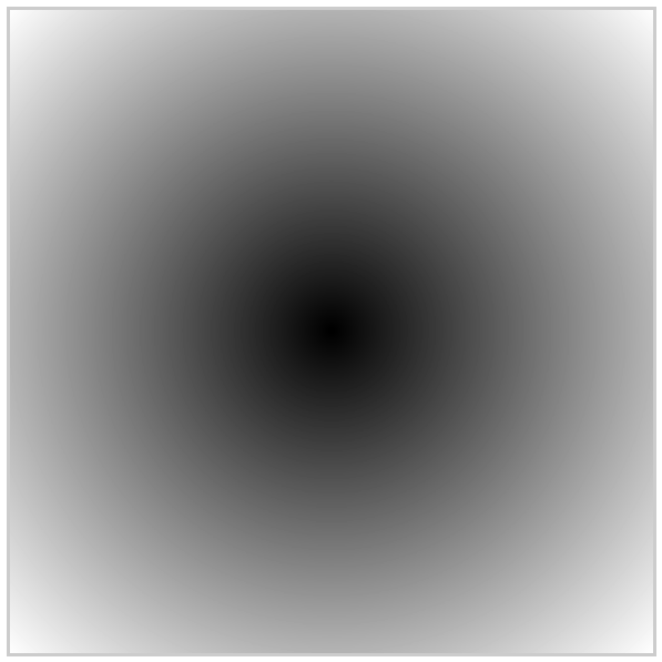
The output from TO can still contain gray values (between 0 and 1) which are not ideal and do not really translate into real-world applications because the presence material in the real world is binary, its either present or absent. There is no intermediate state. Generally, the output from TO are as seen the figures below and are visualized as a 28x28 pixel grid.

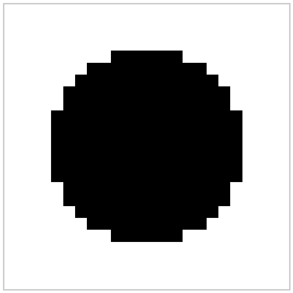
With gray values, approximating the boundary would results in an incorrect volume fraction again, rendering the entire process of topology optimization pointless and even with black and white data and definitive edges, extracting boundary gives the geometry jagged edges. So, a smoothing step in the workflow is necessary.

The geometry smoothing workflow is formulated to handle 2D arrays as the results from the TO are in the form of an image, it can be converted to a 2D array with a size of m×n, where m & n are number of elements in x & y directions. This step mainly consists of two processes. Interpolation and thresholding. The geometry smoothing workflow is presented in the image below.

Interpolation

Interpolation is used in image processing to increase the resolution of the image. In this case, bi-linear interpolation technique is used to increase the resolution of the results to obtain a smooth boundary. Bi-linear interpolation is an extension of linear interpolation for bi-variate data on a rectilinear 2D grid. The schematic of a bi-linear interpolation is shown below.

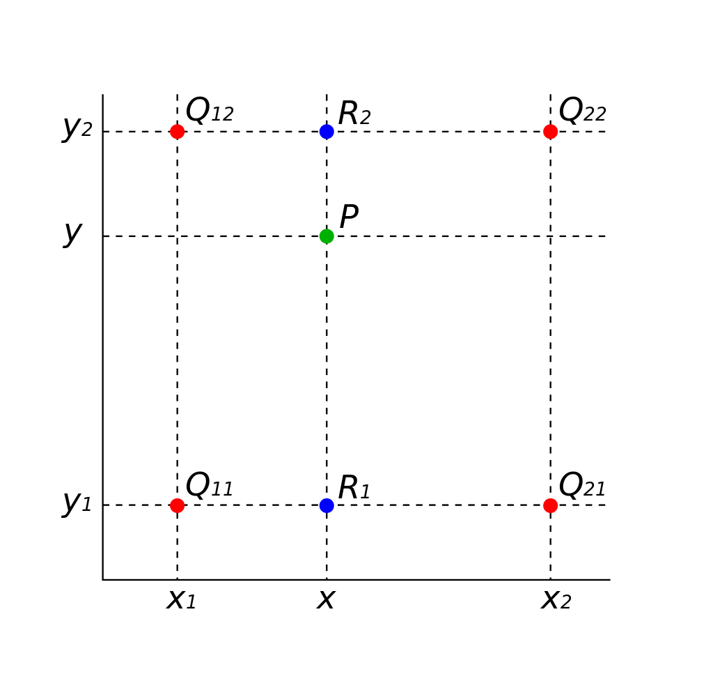
Since, interpolation is a method for generating new data within the range of a know data set, the unknown values can be treated as unknown function f(x, y). The value of f at (x, y) can be calculated by assuming the value of f at four points Q11 = (x1, y1), Q12 = (x1, y2), Q21 = (x2, y1) and Q22 = (x2, y2). For more details on interpolation maths refer to the report.

Thresholding

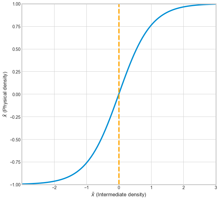
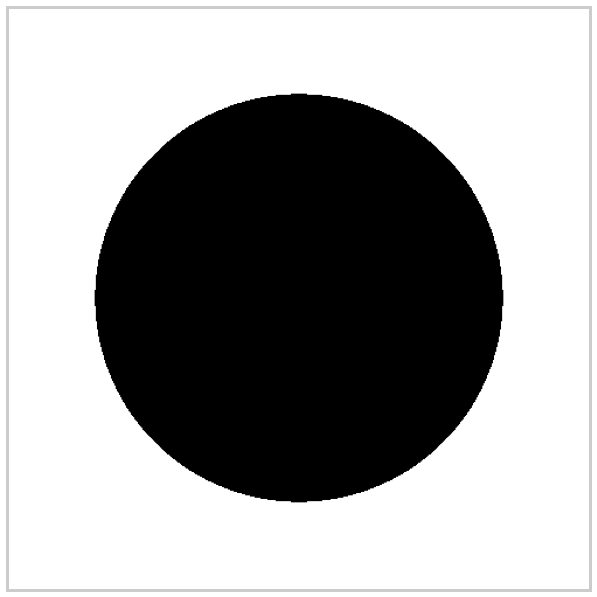
The interpolated nodal data contains intermediate grey values which is not desirable. To get the desired black-and-white results, the interpolated data is run through the Heaviside threshold projection filter which uses a tanh function. The filter can be mathematically presented as seen below.

\begin{equation} \bar{\tilde{x_i}} = \frac{\tanh{(\beta\eta)}+\tanh{(\beta(\tilde{x_i}-\eta))}}{\tanh{(\beta\eta)}+\tanh{(\beta(1-\eta))}}, \end{equation}

where, \(\bar{\tilde{x_i}} \) is the smooth physical density, \(\beta \) is the smoothing factor whose value is the same as the converged \(\beta \) value from topology optimization, \(\tilde{x_i} \) is the interpolated density, and \(\eta \) is the threshold value. The effect of thresholding on the intermediate density data is presented in the below pictures.

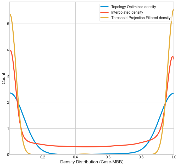
The effect of interpolation and thresholding on the geometry is visualized below.

Geometry Extraction

This phase deals with the extraction of optimized geometry. One of the main challenges of geometry extraction is that the boundaries extracted must be as accurate to the smoothed geometry and the extruded boundaries should not be in need of much post-processing. Considering all of these needs, a workflow was developed which can be seen in below figure.

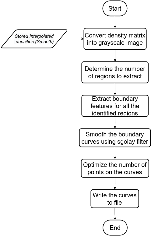
The interpolated smoothed density data is first converted to a grey scale image. The void regions are identified and then extracted. The extracted geometry is then smoothed and the number of nodes are optimized. The optimized curves are then written to a file.

Feature Identification

The regions of interest are identified in MATLAB using regiopnprops. This function is part of the image processing toolbox and it measures the properties of the image regions. The regiopnprops function identifies and differentiates regions in the geometry based on its continuity and density values.

Boundary Smoothing

For smoothing, Savitzky-Golay filters or S-G filters for short is used. SG filter is often used in digital signal processing to eliminate what is termed as small noise variations. S-G filter smooths data by fitting a polynomial to the given set of data using discrete convolution coefficients with a finite impulse response, i.e., it smooths the data while eliminating small noise variations but keeps the overall shape of the curve unaltered. For fitting, S-G filter employs linear least squares method. Mathematically it is described as seen in in the equation below.

\begin{equation}%[!hbt] Y_j = \sum_{i=-m}^{i=m} C_{i}Y_{j+i}, \end{equation}

where, Y is coordinate data, j is the index of the coordinate data, \( C_i \) is the pre- determined convolution co-efficient and m is the range of co-efficient. The filter individually smoothens data for the X and Y co-ordinates separately as it is a 1D filter.

Note: For more detail on how the SG filter is implemented refer to the implementation section of the report and to see how the effect of the SG filter on extracted boundary refer to the discussion and analysis section of the report.

Point density down sampling

The boundary extraction function captures every small detail and hence the number of data points in the coordinate data is high and has a lot of redundancies. This increases the processing and memory resources required to handle data significantly. Therefore the number of points describing the boundary needs to reduce without compromising the geometry. To achieve this the Recursive Douglas-Peucker Polyline Simplification Algorithm is used. This function down samples and simplifies the boundary coordinate data without compromising the final geometry. The pseudo code for the line simplification algorithm is give below.

    
    Ramer-Douglas-Peucker Algorithm

    function RDP(PointsList, epsilon)
      dmax = 0
      end = length(PointList)

      for {i = 2 : (end -1)}
        d = perpendicularDistance(
          PointList[i], 
          Line(PointList[1], 
          PointList[end]))

        if {d > dmax}
          index = i
          dmax = d
        endIf
      endFor

      ResultList = empty;
      if{dmax > epsilon}
        recursive1 = RDP(PointList[1...index], epsilon)
        recursive2 = RDP(PointList[index...end], epsilon)
        ResultList={recursive1[1:length(recursive1)-1],
                    recursive2[1:length(recursive2)]}
      else
        ResultList = {PointList[1], PointList[end]}
      endIf
    return ResultList;
    
    

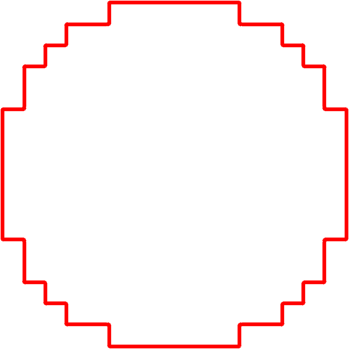
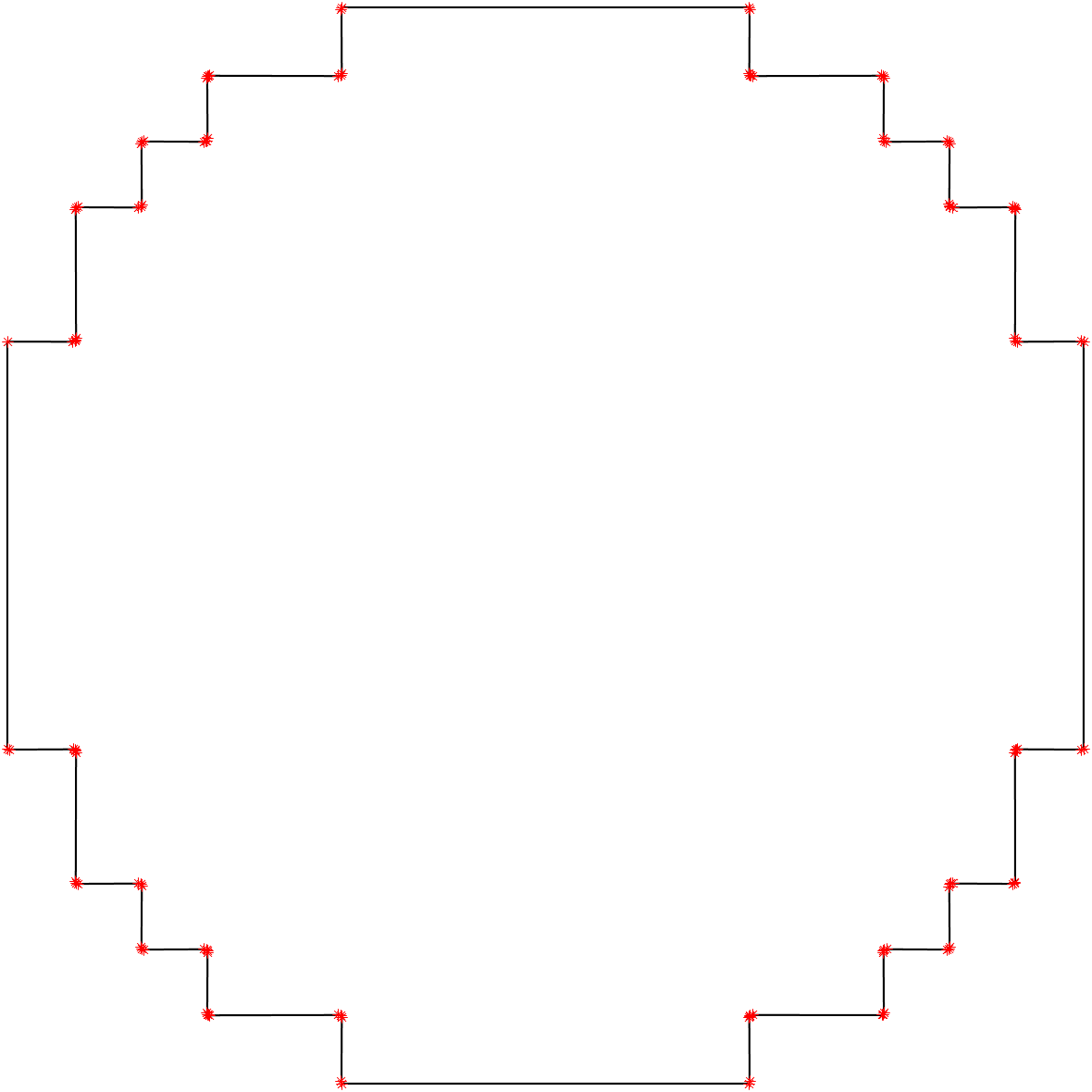
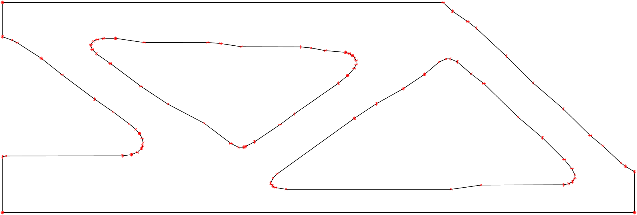
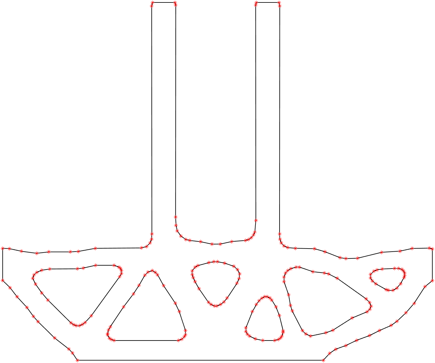
The effect of RDP algorithm on the boundary coordinate data is shown in the figures below. The figure on the left has 12577 points and the one on the right has 36 points. The 'simplified' version of the co-ordinates of these boundaries are written onto text files which can then be imported on to a CAD software to make a 2D surface or an extruded 3D geometry.

Results

This chapter presents the results of the implemented workflow discussed in the previous sections. Here, two numerical examples are presented.An MBB beam, a classical test case in TO and a T-shaped beam with a hole is also tested which is a complex case as the initial geometry is asymmetric and has two loads acting on it.

Material Properties

The material parameters for each of the numerical examples executed is as follows: Young's modulus \( E_0 \) is 1, \( E_{min} \) is the Young's modulus for the void regions is \( 1e^{-9} \) , Poisson's ratio \( \nu \) of 0.3, a filter radius of 0.03 \(\times \) nelx, where nelx is the number of elements in the x-direction. a penalization factor of 3 and an interpolation value of 8. All the cases are solved for the compliance minimization criteria.

MBB Beam

Boundary Conditions

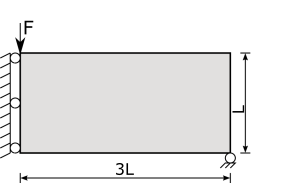
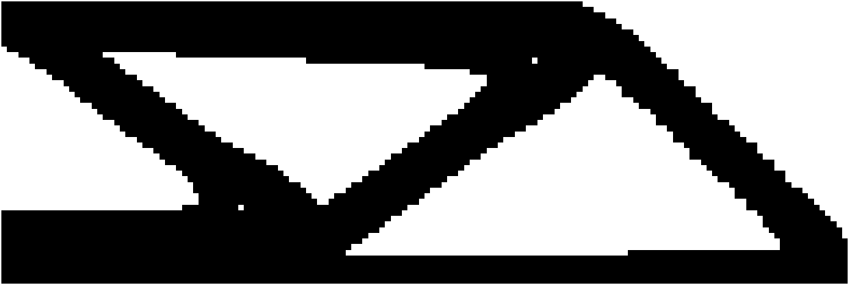
Phase 1: TO

Phase 2: Geometry Smoothing

Phase 3: Geometry Extraction

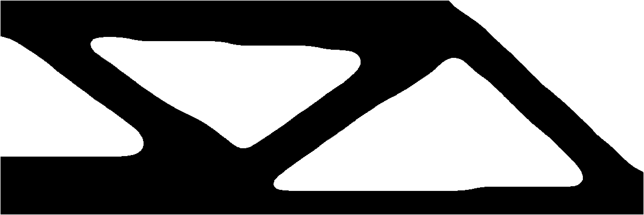
T Beam with Hole

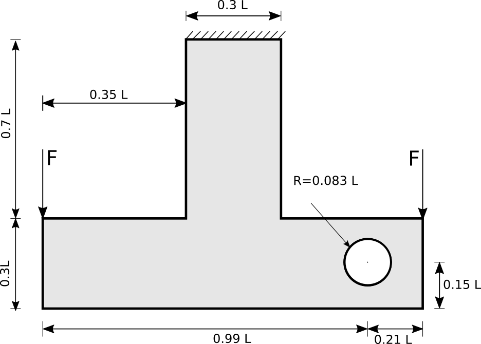
Boundary Conditions

Phase 1: TO

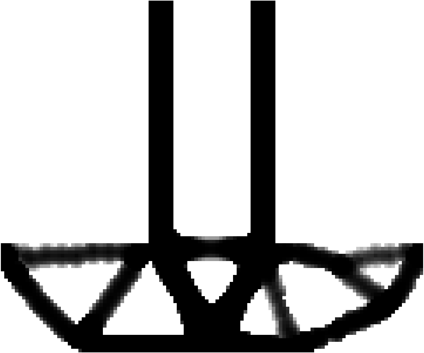
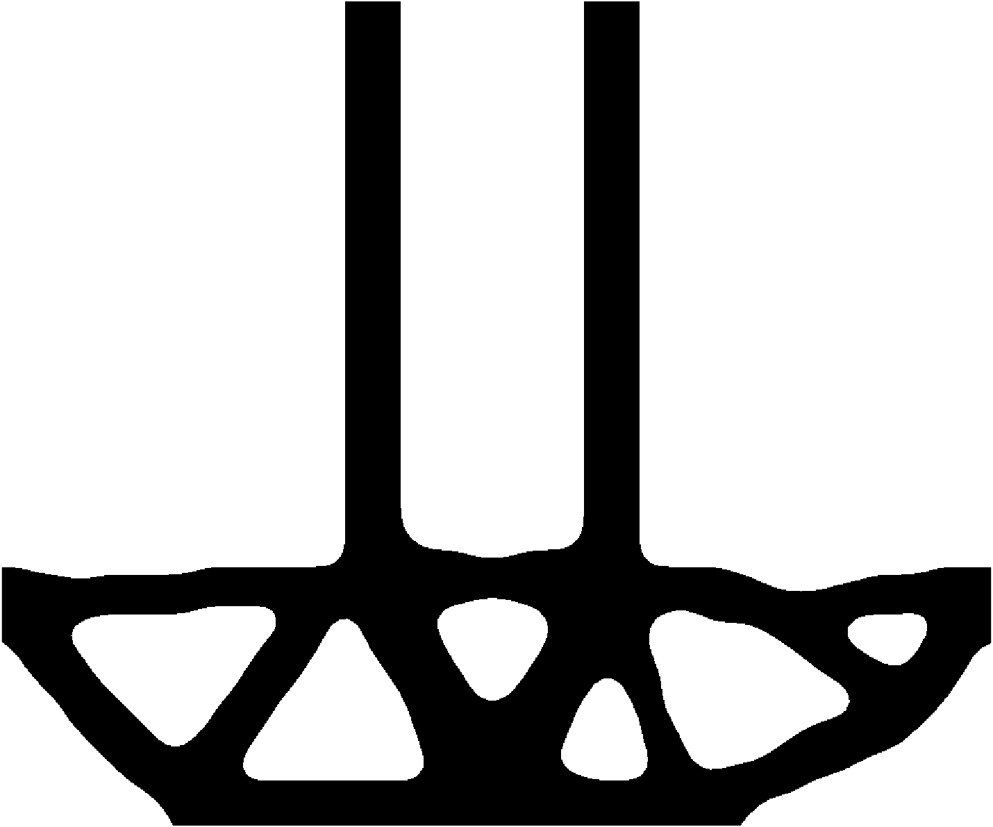
Phase 2: Geometry Smoothing

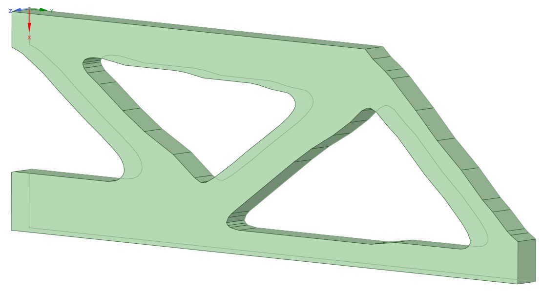
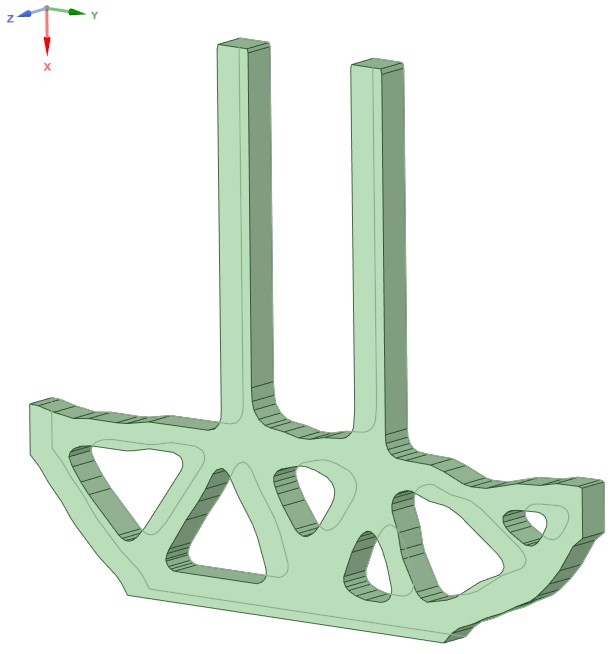
Phase 3: Geometry Extraction

Note: Additional numerical examples such as Half-wheel, cantilever beam, L-shaped beam etc have been executed and documented in Appendix B of the report.

Additional Details

Result Metrics

Case	Target Volume fraction	Optimized Compliance (Unsmooth)	Post Processed Data (Smooth)
			Volume fraction	Compliance
MBB Beam	0.5	191.4968	0.5088	195.243
T Beam with hole	0.25	326.2442	0.2484	301.733

Limitations

• Works Only with 2D solvers
• Manual geometry extrusion, i.e., converting 2D data to 3D geometry is performed in a separate software
• Fails at low volume fractions and need manual tweaks for the suggested work around. See 6.6.2 Evaluation of extreme scenarios in the report.

Outlook

• SIMP in combination with Heaviside filter give good starting point to post- process TO results.
• Interpolation combined with threshold projection filter helps remove jagged edges and outputs smooth geometry with acceptable deviation.
• S-Golay filter with RDP algorithm extracts a usable smooth boundary data to transfer to a CAD software and get a manufacturable 3D geometry.
• Most of the workflow is automated from input data to boundary extraction. 3D geometry generation is done manually.
• It is a generalized approach and the methodology can be adopted for rapid proto-typing.
• Possible Improvements
• Code can be made faster when written in languages such as C++, FORTRAN, etc.
• Workflow can be adopted for 3D geometry